Database Detective: Discogs


Table of Contents
- Building the database
- Questions and answers
- A brief history of recorded audio, as told by Discogs
- A galaxy of genres, a sea of styles
- Questions and answers, pt. 2
- Conclusion
Chapter 1: Building the database
Motivation
As a record collector, I've found that one of the best places to find and purchase albums is through the Discogs online marketplace.
But Discogs is more than a marketplace for vinyl, CDs, and audio media of all kinds. It's also the world's largest online music database, containing information about over 15 million releases, 8 million artists, and nearly 2 million labels.
The Discogs model is sort of like Wikipedia. Registered users submit new releases into the website and include information about the artist, title, label, format, tracks, genre, and style. Volunteer moderators check for inaccuracies and correct them. All of the data on Discogs is generated freely by its users.
Discogs makes its data available for download under the Creative Commons No Rights Reserved license through monthly XML file releases. As of June 2022, the monthly data release was ~11 GB in size across four XML files. These XML files are nearly impossible to open in a text editor, but even if you could open them, their contents are difficult to decipher. Ideally, I could somehow parse the XML, then use the result to build a SQL database for quick access.
Standing on the shoulders of giants
Luckily, I discovered discogs-xml2b, an open-source project containing programs designed to convert the Discogs XML data files into a database. First, I downloaded the four XML files in the latest data release. Next, I simply dragged each XML file onto discogs-xml2b's .NET-based parser program, which generates a total of ~20 comma-separated-value (CSV) files. The CSVs resemble spreadsheets in which each row corresponds to a release, artist, or label, and each column contains information about that entity.
The CSV files, which are already structured like database tables, are then inserted into a database schema (currently discogs-xml2b has support for PostgreSQL, MySQL, MongoDB, or CouchDB). I chose to build a PostgreSQL database. After installing PostgreSQL and the useful database administration tool pgAdmin onto my computer, I got myself acquainted with how to use PostgreSQL. I configured my Windows machine to allow me to access the database from the command line, created a user, and created a fresh database named discogs.
Next came importing the CSV files into the fresh database. The discogs-xml2b repo contains Python scripts designed to accomplish this task. Since I was using PostgreSQL as my database, I first had to install the psycopg2 library into my Python environment. I also had to add my PostgreSQL credentials (username and password) to a configuration file. Since I'm using a Windows machine, I had to do a little bit of tinkering with the Python programs and shell commands to get them to run properly. For example, the repo suggests you run a command like the following:
python3 postgresql/psql.py < postgresql/sql/CreateTables.sqlThe < operator here redirects the contents of the SQL script as the standard input into the Python script psql.py. But this syntax isn't supported in Windows PowerShell. Instead, I had to run the command like this:
Get-Content postgresql/sql/CreateTables.sql | python postgresql/psql.pyAlternatively, one could manually connect to the database and run each SQL script without using the Python wrapper, either from the command-line or from pgAdmin.
After creating the tables, discogs-xml2b provides a useful python script for importing each CSV file into its corresponding table. Here I encountered my first major hiccup. I noticed that a few of the CSV files caused errors and could not be successfully imported into the database: artist_url, release_track, and release_track_artist. This was due to errors in the CSV files themselves, which could probably be traced back to issues in the XML files. While I could have spent the time to fix this problem at the source, I wasn't interested in the URLs or the information about the individual tracks on the albums, so I decided to abandon this unnecessary data. I also identified a few more CSVs that were superfluous (e.g. image sizes and YouTube video URLs). I wanted to delete these CSVs and remove the corresponding data from the database.
But this meant that the database schema intended by discogs-xml2b would need to be modified. I inspected and edited the SQL scripts CreateTables.sql, CreatePrimaryKeys.sql, CreateFKConstraints.sql, and CreateIndexes.sql in order to factor out the erroneous and unnecessary data from the database schema. Once convinced I'd done this correctly, I deleted the unneeded CSV files, dropped the database, and rebuilt it from scratch using the modified database schema. In the end, the schema had 17 tables. I created the tables, imported the CSV data into the tables using the Python script, and ran the modified scripts to create the primary keys, foreign key constraints, and indexes.
Getting my hands dirty
My discogs database was ready to investigate! Or so I thought.
I went through each column in each table and wrote a small guide to reference as I did my analyses. In doing so, I identified a few issues. First, a couple columns contained useless information, so I dropped them. A couple more columns were fully NULL and didn't seem useful based on their names, so I dropped them. Finally, a couple columns had names implying they should have contained useful information, but all of the values were NULL.
Luckily due to some redundancy the database contained enough information to fill in what was missing in some cases. For example, I was able to fill in the fully-NULL release_label.label_id (a one-to-many foreign key of label.id) based on the equivalence of release_label.label_name and label.name. And I was able to set the value of the fully-NULL release.main to signify that a given release was the "main" release amongst its versions using master.main_release. Performing these quality checks removed distracting information and allowed me to be as confident as possible that the database was correct.
As I scanned over the guide I had written about the tables and their columns, my mind flooded with questions that could be answered with the dataset. I wrote my questions down, and one by one I began writing queries to answer each question.
I was hooked. Answering one question motivated more related questions. I felt like a detective. Fact by fact, I learned an incredible amount of information. Most of it was completely useless, but I was fascinated.
What were the most successful albums and artists of all time? Why can no one agree on how to spell Tchaikovsky? What was the story behind the first recording ever made, back in 1860? What kind of audio formats are Flexi-disc, Minidisc, and SACD? How do genres and styles relate to each other? Who is Caliph Mutabor, and why do they have over 1500 musical aliases? What was the story behind Defaultest 93, a digital release with 10^188 audio files – essentially a glorified computer virus? Did a Russian person really make an 85-cassette collection of hard techno? Did a Hungarian artist really release make an 80-CDr album of harsh noise music? And did My Chemical Romance really release a live album for the Sony PlayStation Portable (PSP)?
Believe it or not, by hammering away boring SQL queries, I found enough conversation starters to last me years. In the coming chapters, I'll explain what I learned.
Chapter 2: Questions and answers
Making the qualitative quantitative
I've always loved music. I was a college radio DJ for about 4 years, which gave me a glimpse into a small part of its massive world. But how much do I really know about music as an industry? About the history of putting musical releases into the hands of listeners?
The beautiful thing about data analysis is that it allows you to answer questions about the real world. As virtual as it may seem, the content of the Discogs database is real: its data corresponds to real people who often poured their heart and soul into making real artistic works that others could experience. I had many questions that I wanted to answer about the musical world, so I went to work.
Just a quick technical note before we get started: the Discogs database contains primarily qualitative information. Across the 17 tables, there are about 30 text columns: names, descriptions, categories, notes, etc. Quantitative information is actually quite scarce, with the only numerical columns being the year of the release and the number of pieces of media in the release (i.e. a double album is 2). The most straightforward way to make the qualitative information amenable to quantitative analysis is to aggregate by counting. And one of the most interesting ways to use aggregation is to find the extremes (e.g. top 10 lists). With that in mind, let's jump in.
What master recording has had the most releases?
To make this clearer, I should explain that Discogs not only tracks different recordings, but it also keeps track of the multiple releases of the same recording. Why should a recording have multiple releases? For example, this occurs when it's released in different regions, on different record labels, on multiple audio formats, or when it's reissued. But for any recording with multiple releases, there is only one "master," which refers to the original recording from which all of the copies are made.
Since the Discogs database links each release to its master recording, we can ask: What master recording has had the most releases? As I go, I'll include the SQL query in a collapsible section if you're interested:
SQL Query
SELECT
  m.id,
  m.title,
  m.year,
  q1.releases
FROM master AS m
  INNER JOIN (SELECT
                master_id,
                COUNT(*) AS releases
              FROM release
              WHERE master_id IS NOT `NULL`
              GROUP BY master_id
              ORDER BY releases DESC
              LIMIT 10) AS q1
    ON m.id = q1.master_id
Result:
| ID | Title | Year | Releases |
|---|---|---|---|
| 10362 | The Dark Side Of The Moon | 1973 | 1141 |
| 23934 | Sgt. Pepper's Lonely Hearts Club Band | 1967 | 1052 |
| 4300 | Untitled | 1971 | 949 |
| 24047 | Abbey Road | 1969 | 860 |
| 4170 | Led Zeppelin II | 1969 | 857 |
| 11703 | Wish You Were Here | 1975 | 849 |
| 45526 | Rubber Soul | 1965 | 817 |
| 11329 | The Wall | 1979 | 781 |
| 46402 | The Beatles | 1968 | 771 |
| 45284 | Revolver | 1966 | 761 |
As you can see, this list is dominated by the titans of classic rock: Pink Floyd, The Beatles, and Led Zeppelin. The albums have become culturally iconic not only for the music but also the cover art. You also probably noticed that all of these albums were released in the '60s and '70s, which means they benefit from having had up to fifty years to be reissued. By the way, if you didn't recognize the album called Untitled, that's the official name of Led Zeppelin's fourth studio album, which most people call Led Zeppelin IV. But Pink Floyd's The Dark Side of the Moon takes home first prize. Dark Side has been released in over fifty countries, on eight media formats, and in association with over a hundred companies. The query that returns this result is shown below
SQL Query
SELECT
  COUNT(DISTINCT country) AS distinct_countries,
  COUNT(DISTINCT format)  AS distinct_formats,
  COUNT(DISTINCT label)   AS distinct_labels
FROM
  (SELECT
     r.id,
     r.title,
     r.released,
     r.country,
     rf.name       AS format,
     rl.label_name AS label
   FROM
     (SELECT *
      FROM release
      WHERE master_id = 10362) AS r
     INNER JOIN release_format AS rf
       ON r.id = rf.release_id
     INNER JOIN release_label AS rl
       ON r.id = rl.release_id) AS q1;
Obviously the previous analysis is biased by the amount of time since the initial release. The longer it's been since an album was first released, the more re-releases it should have. What if we normalize the number of releases by the number of years since the initial release? We could call the quantifier "releases per year since initial release," but I'll also add a constant of 14 years into the denominator, which accomplishes two things: 1) It prevents a division by zero error for albums released this year, and 2) It prevents albums released recently from dominating the analysis.
SQL Query
SELECT
  m.id,
  m.title,
  m.year,
  q1.releases,
  2036.0 - m.year                 AS years_til_2036,
  q1.releases / (2036.0 - m.year) AS year_norm
FROM master AS m
  INNER JOIN (SELECT
                master_id,
                COUNT(*) AS releases
              FROM release
              WHERE master_id IS NOT `NULL`
              GROUP BY master_id) AS q1
    ON m.id = q1.master_id
ORDER BY year_norm DESC
LIMIT 10;
Result:
| ID | Title | Year | Releases | Year Norm |
|---|---|---|---|---|
| 10362 | The Dark Side Of The Moon | 1973 | 1141 | 18.11 |
| 1268453 | Polygondwanaland | 2017 | 336 | 17.68 |
| 23934 | Sgt. Pepper's Lonely Hearts Club Band | 1967 | 1052 | 15.25 |
| 13814 | Nevermind | 1991 | 685 | 15.22 |
| 4300 | Untitled | 1971 | 949 | 14.60 |
| 11703 | Wish You Were Here | 1975 | 849 | 13.92 |
| 11329 | The Wall | 1979 | 781 | 13.70 |
| 24047 | Abbey Road | 1969 | 860 | 12.84 |
| 4170 | Led Zeppelin II | 1969 | 857 | 12.79 |
| 8883 | Thriller | 1982 | 636 | 11.78 |
Normalizing this way adds a lot more diversity to the list. Nirvana's Nevermind was released relatively recently in 1991, but it's still managed to rack up 685 releases since then, and Michael Jackson's Thriller scored 636 releases since its 1982 debut.
You're probably wondering about Polygondwanaland, and there's a good explanation for how it managed to achieve 336 releases since it was made in 2017. When King Gizzard and Lizard Wizard initially released it, they made the master audio files available to download for free on their website. But they went even further than that: they encouraged their fans to make copies of the record and sell it, providing digital-, CD-, and vinyl-ready audio files, as well as album art files. To quote them: "This album is FREE. Free as in, free. Free to download and if you wish, free to make copies. Make tapes, make CD's, make records. … Ever wanted to start your own record label? GO for it! Employ your mates, press wax, pack boxes. We do not own this record. You do. Go forth, share, enjoy." The result? Polygondwanaland has been released in over twenty countries, on nine media formats, on over a hundred distinct labels. That's one way to spread the word.
What artist has the most master recordings attributed to them?
SQL Query
SELECT
  q1.artist_id AS id,
  a.name,
  q1.masters
FROM
  (SELECT
     artist_id,
     COUNT(*) AS masters
   FROM master_artist
   GROUP BY artist_id
   ORDER BY masters DESC
   LIMIT 8) AS q1
  INNER JOIN artist AS a
    ON q1.artist_id = a.id;
Result:
| ID | Name | Masters |
|---|---|---|
| 95546 | Wolfgang Amadeus Mozart | 5951 |
| 95544 | Ludwig van Beethoven | 5413 |
| 95537 | Johann Sebastian Bach | 4984 |
| 999914 | Pyotr Ilyich Tchaikovsky | 2738 |
| 283469 | Franz Schubert | 2498 |
| 304975 | Johannes Brahms | 2455 |
| 108568 | Joseph Haydn | 2147 |
| 262940 | The London Symphony Orchestra | 1957 |
| 192325 | Frédéric Chopin | 1785 |
| 27518 | Elvis Presley | 1666 |
In the case of most distinct albums by artist, classical composers dominate. The reason for this is threefold: First, they were genuinely prolific – not being limited by the speed of recording but by how quickly they could write their compositions onto paper. Secondly, their compositions have been recorded and released essentially since the dawn of recorded audio in the late 19th century. And finally, because the copyright duration of composed music only lasts 70 years beyond the author's death, their works are all in the public domain. This means that their works can be freely used and recorded by any number of musicians, and there is no "definitive" recording of any of their compositions. Still, the King rounds out this list at spot #10.
What artist has the most name variations?
SQL Query
SELECT
  a.id,
  a.name,
  q1.variations
FROM artist AS a
  INNER JOIN (SELECT
                artist_id,
                COUNT(*) AS variations
              FROM artist_namevariation
              GROUP BY artist_id
              ORDER BY variations DESC
              LIMIT 10) AS q1
    ON a.id = q1.artist_id
ORDER BY variations DESC;
Result:
| ID | Name | Variations |
|---|---|---|
| 151641 | Traditional | 10420 |
| 320156 | Folk | 6334 |
| 967691 | Anonymous | 2134 |
| 999914 | Pyotr Ilyich Tchaikovsky | 1044 |
| 779927 | Lennon-McCartney | 918 |
| 746270 | Robin Gibb, Barry Gibb & Maurice Gibb | 908 |
| 838295 | Большой Симфонический Оркестр Всесоюзного Радио | 872 |
| 476910 | Holland-Dozier-Holland | 825 |
| 142502 | Bacharach And David | 602 |
| 975170 | Björn Ulvaeus & Benny Andersson | 599 |
This analysis tells us a few things. First, Discogs uses name variations to keep track of the different ways people refer to 'Traditional' and 'Folk' music (i.e. music that has been handed down in a culture) as well as 'Anonymous' music, when the identity of the artist is not known.
Second, this analysis tells us that people really, really cannot agree on how to spell Tchaikovsky's name, with over a thousand variations. Apparently, this is because when Russian names are transliterated from Cyrillic letters into Roman letters, many different spellings can result due to the different rules of pronunciation for each language. The 7th place entry on this list translates to the Tchaikovsky Symphony Orchestra, and it has the same explanation.
Finally, this analysis tells us that record companies also can't agree on how to spell the name of songwriting teams (e.g. Lennon-McCartney vs. Lennon & McCartney). The songwriting teams that made this list are the ones behind the Beatles (Lennon-McCartney), the Bee Gees (the Gibb brothers), Motown Records (Holland-Dozier-Holland), ABBA (Björn Ulvaeus & Benny Andersson), and the songwriting duo of Burt Bacharach and Hal David.
Now that we've answered a few basic "Top 10"-style questions let's move on to a different topic. I'll answer even more questions in the final chapter.
Chapter 3: A brief history of recorded audio, as told by Discogs
What is the earliest known audio recording?
SQL Query
SELECT
  id,
  title,
  released,
  country
FROM release
WHERE released LIKE '1%'
ORDER BY released
LIMIT 5;
Result:
| ID | Title | Released | Country |
|---|---|---|---|
| 1289378 | Au Clair De La Lune | 1860 | France |
| 5695167 | Experimental Talking Clock | 1878 | US |
| 8532114 | Mary Had A Little Lamb | 1878 | US |
| 4275659 | A Little Ship Was On The Sea | 1889 | Germany |
| 2583289 | Electric Light Quadrille | 1889 | US |
Recorded audio begins with Édouard-Léon Scott de Martinville, who invented a device he called the phonautograph in 1857. It funneled sound through a cone onto a vibrating membrane attached to a stylus, which would then trace the membrane's vibrations onto a rotating cylinder covered with soot. In 1860, Scott recorded part of a French folk song titled 'Au Clair de la Lune,' which remains the earliest clearly recognizable record of the human voice. However, because he didn't have a method of playing back the recording, it wasn't until 2008 that researchers were able to scan the cylinder to convert the recording into audio.
In 1877, Thomas Edison invented the phonograph, which recorded sound onto a soft tinfoil sheet wrapped around a cylinder. Unlike Scott's phonautograph, the phonograph cylinder could be used to both record and reproduce sound. However, his earliest recordings were extremely fragile and could not be preserved. His first recording that still exists is of the nursery rhyme 'Mary Had A Little Lamb' in 1878.
Months after Edison invented the phonograph, Frank Lambert – a French immigrant to America – created a phonograph-inspired device that utilized a lead cylinder rather than soft tinfoil. Due to its durability, his recording 'Experimental Talking Clock' from 1878 actually predates Edison's oldest surviving record and can still be played with its own mechanism.
Ten years later, in 1888, Emile Berliner invented the gramophone, which functioned by imprinting grooves onto a flat disc of rigid latex made from tree sap. His first recording was of a woman reading the poem 'A Little Ship Was On The Sea.'
By the 1890s, phonograph and gramophone-inspired recording techniques began to take off, and selling recorded audio became a profitable business endeavor. But while cylinders died out, discs succeeded. Around 1895, discs made of shellac – a resin secreted by bugs – became the standard material and were mainly designed to be spun at 78 rotations per minute (RPM).
The rise and fall of audio formats
In 1948, Columbia introduced 12-inch-diameter discs made of polyvinyl chloride acetate, or simply vinyl. With smaller grooves and a slower rotation speed of 33⅓ RPM, they could be played for much longer and became known as "long-play" records or LPs. The following year, RCA Victor introduced 7-inch-diameter vinyl records designed to be played at 45 RPM, which became referred to as simply "45's". These two vinyl formats – the 12-inch LP and the 7-inch 45 – went on to become the dominant forms of commercially-available audio media for nearly thirty years until the rise of cassettes in the late 70's and the introduction of CDs in the late 80's.
Around 2010, digital distribution of music files became the predominant form of music releases via services like iTunes, Spotify, and Apple Music. Interestingly, while CDs continue to fall in popularity, vinyl and cassette releases have actually increased since around 2010, signaling a revival of interest in and demand for analog formats.
Because Discogs tracks the format of each release and the year it was released, we can query this information and visualize the results using Tableau. To do so, I connected my Tableau application directly to my local PostgreSQL database and used a custom SQL query as a data source.
SQL Query
SELECT
  q1.format,
  q1.released_year,
  COUNT(*)
FROM
  (SELECT
     to_date(left(r.released, 4), 'YYYY') AS released_year,
     rf.format
   FROM release AS r
     INNER JOIN (SELECT
                   release_id,
                   MAX(name) AS format
                 FROM release_format
                 GROUP BY release_id) AS rf
       ON r.id = rf.release_id) AS q1
GROUP BY q1.format, q1.released_year;
To visualize this information, I chose an "area" graph because it not only shows both the rise and fall of each format but also the overall increase in musical releases per year.
Lesser-known formats
While we're on the topic of audio formats, I'd like to shine some light on some lesser-known audio formats that didn't quite stand the test of time. By using the same data source as the previous visualization, I was able to create the following line plot:
Behind the scenes, magnetic tape-based recording was massively important to the process of audio production from around 1940 and onward. Initially, this utilized a 'reel-to-reel' design in which a relatively wide (at least ¼ inch) recording tape was spooled between two reels. In the early 1950s, reel-to-reel tape machines began being sold for home usage, and record companies sold albums on pre-recorded tape reels. Although its excellent sound fidelity made it a favorite format of audiophiles for decades, reel-to-reel tape players were expensive and difficult to use, and pre-recorded tape reels took much longer to produce than vinyl.
The better-known but ultimately unsuccessful tape format was the 8-Track Cartridge. 8-Track was developed in 1964 about a year after the Philips microcassette (a.k.a. cassette) and utilized a fairly similar conceptual design. After being offered as optional upgrade on Ford cars beginning in 1966, 8-track gained massive popularity that lasted well into the 70's, but it was eventually outcompeted by the cassette.
Flexi-disc was a type of vinyl disc record that was much thinner and more flexible than normal vinyl discs. Their flexibility meant that flexi-discs could be bound inside of magazines and booklets yet still be played on normal record players. Flexi-discs filled this niche from around 1960 to 1990 until the CD exploded in popularity and became the preferred format for including recorded audio in print media. Interestingly, flexi-discs have seen a resurgence in popularity beginning in 2010.
Lathe-cut records are discs in which the groove is cut by rotating the disc underneath a needle, instead of pressing the groove into hot vinyl with a metal stamper. Lathes have been used since at least the 1920s to cut the single "master" record (typically onto a lacquer-coated aluminum disc) from which a negative-image metal stamper is created in order to mass-produce pressed records. But in the past decade, lathes have been used to cut polycarbonate discs for small record runs (e.g. less than 200 records). This has become a popular technique among independent record labels and artists that embrace the "do it yourself" mantra.
Finally, the MiniDisc and Super Audio CD (SACD) formats were designed to improve upon cassettes and CDs, but they weren't accepted by the mainstream market. Introduced in 1992, MiniDiscs were impressively small at about 3 x 3 inches, could be made and edited quickly, and had superior anti-skip technology compared to CDs. Introduced in 1999, SACD allowed surround sound and higher audio quality compared to CDs. Although these technical advantages weren't enough to allow MiniDiscs or SACDs to achieve major commercial success, neither format is completely dead. SACDs continue to be released, and MiniDisc has experienced a small revival.
Chapter 4: A galaxy of genres, a sea of styles
The genres and styles with the most releases
Perhaps the most difficult topic to tackle in music is its stunning stylistic diversity. In the Discogs database, each release must be tagged with at least one genre and at least one style. Genres function as super-categories; there are only fifteen. On the other hand, styles are designed to be sub-categories of a single genre, and there are 602 total styles.
Approaching the Discogs database, I had a couple different ideas about how to make genres and styles amenable to quantitative analysis. One obvious idea was to find out which genres and styles had the most releases. In order to visualize the results, I used Tableau to create simple bar charts directly from the results of SQL queries against my local PostgreSQL database. First, let's take a look at the number of releases in each of the fifteen genres:
Rock, Electronic, and Pop are by far the largest genres by number of masters. Which styles have the largest number of releases? Since each style is a sub-category of a genre above, we can color each bar according to its genre:
It may surprise you to see that House music is the style with the most releases. Actually, Discogs was initially founded with the goal of being the most comprehensive database of Electronic music, and House is a style of Electronic music that is infamously diverse with numerous sub-styles. Furthermore, House (and most Electronic Dance music) is typically released via numerous singles rather than full albums, which serves to further boost the total count of its releases.
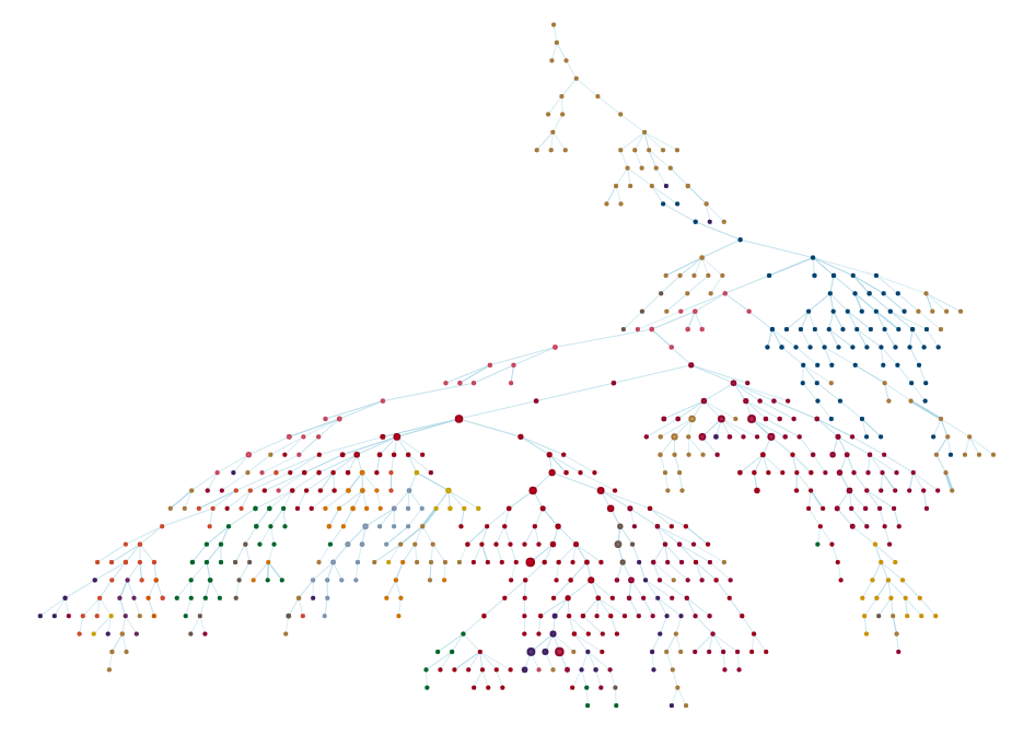
Building a map of stylistic space
While the previous analysis was interesting, I wasn't satisfied. One of the coolest things about musical styles is their interconnectedness. As a style flourishes, individuals working within the style innovate new sub-styles, which go on to spawn their own sub-styles, forming a "family tree" of music. I wanted to find a way to visualize this fact using the Discogs database. From an analytical perspective, this turned out to be tricky, but the final result was beautiful.
To visualize the interconnectedness of genres and styles, I focused on the concept of co-occurrence. You see, releases submitted to Discogs are required to be tagged with at least one genre and style, but many releases are tagged with multiple genres and styles. If one release is tagged with two different styles – say, Psychedelic Rock and Prog Rock – it probably means the two styles are related in some way. And by knowing how related each pair of genres or each pair of styles was, I could begin to build a map of stylistic space in music.
First, I needed to count the co-occurrences of genres and styles (separately) in the database. I was able to do this with a type of SQL query called a self-join, which you can see below for styles:
SQL Query
SELECT
  a.style  AS g1,
  b.style  AS g2,
  COUNT(*) AS cnt
FROM master_style AS a
  INNER JOIN master_style AS b
    ON a.master_id = b.master_id AND a.style < b.style
GROUP BY a.style, b.style;
Once I had the co-occurrences, I faced a quantitative problem. Let's say I know that two styles – say, Ambient and Downtempo – co-occur exactly 7000 times. Is that a lot? Well, it depends on how many releases are tagged as Ambient or Downtempo to begin with. If there are only 7000 releases tagged as either Ambient or Downtempo, then that means that every single release tagged as Ambient is also tagged as Downtempo – they would be 100% connected. But if there are 14000 releases tagged as either Ambient or Downtempo, then they would be 50% connected (7000 / 14000). This fraction is called the Jaccard index, and it provides an intuitive and effective quantifier of co-occurrence while normalizing for the number of occurrences.
Now that I knew how connected the genres and styles were, it was time to build a graph. Not a graph as in a plot of a mathematical function, but a graph as in graph theory. In the mathematical field of graph theory, graphs are network-like objects in which nodes are connected by edges, and the edges are often assigned weights, i.e. values reflecting the strength of each connection. In the current analysis, the nodes are the musical genres (or styles), and the edge weights represent how often a particular pair of genres (or styles) is co-tagged on a single release.
Once I'd built my first graph, I encountered the final challenge in this analysis. To put it succinctly, genres and styles are a little too connected. In fact, every genre co-occurred with every other genre at least once. For the case of genres, this doesn't cause major issues because the graph only has 15 nodes and 105 edges. But the visualization of this kind of graph isn't very informative; it simply looks like an overly complicated spiderweb. And for the case of the 602 styles, each style co-occurred with about 25% of the other styles resulting in a graph with a staggering 45000+ edges. Not only will this look like a mess, but attempting to visualize such a graph will crash most computers.
Fortunately, there are methods for "pruning" graphs. Naively, one may imagine that an effective way of pruning graphs would be to simply delete any edges whose weight is beneath a certain threshold value. While this can be effective, the choice of weight threshold is arbitrary, and it often results in disconnected graphs. Instead, I chose to find the so-called maximum spanning tree of the graph. Put simply, the maximum spanning tree is the smallest set of edges that connects all of the nodes in the graph while having the largest sum of edge weights. In other words, the maximum spanning tree is as sparse as possible (fewest connections) while keeping everything connected, but the connections that are included are the strongest – and hopefully the most meaningful.
To carry out the rest of this analysis and visualize the results, I used Python and JavaScript. The sequence is roughly as follows:
- Import the result of the SQL query that returned the co-occurrences and occurrences of genres and styles into Python as pandas dataframes.
- Calculate the Jaccard co-occurrences.
- Using
networkx, construct a graph in which the nodes are genres/styles, and the edge weights are the Jaccard co-occurrences. - Utilize the
networkxfunctionmaximum_spanning_treeto create a pruned version of the initial graph. - Export the node and edge information into JSON files.
- Import the JSON files and visualize the graphs in the browser using
vis-network.
This provides an interactive visualization in which you can zoom, move nodes, and play to your heart's content. Please check it out using this link or click the picture below!
Chapter 5: Questions and answers, pt. 2
What master recording has the longest name?
SQL Query
SELECT
  id,
  title,
  length(title) AS title_length
FROM master
ORDER BY title_length DESC
LIMIT 10;
I won't include all of the results here (it would take up a bit too much space), but the longest album title has 552 characters: It's an album of remixes by the band Soulwax called Most Of The Remixes We've Made For Other People Over The Years Except For The One For Einstürzende Neubauten Because We Lost It And A Few We Didn't Think Sounded Good Enough Or Just Didn't Fit In Length-Wise, But Including Some That Are Hard To Find Because Either People Forgot About Them Or Simply Because They Haven't Been Released Yet, A Few We Really Love, One We Think Is Just OK, Some We Did For Free, Some We Did For Money, Some For Ourselves Without Permission And Some For Friends As Swaps But Never On Time And Always At Our Studio In Ghent.
What artist is a member of the most groups?
SQL Query
SELECT
  a.id,
  a.name,
  q1.instances AS groups
FROM artist AS a
  INNER JOIN (SELECT
                member_artist_id,
                COUNT(*) AS instances
              FROM group_member
              GROUP BY member_artist_id
              ORDER BY instances DESC
              LIMIT 10) AS q1
    ON a.id = q1.member_artist_id
ORDER BY instances DESC;
Result:
| ID | Name | Groups |
|---|---|---|
| 837308 | Frankie Fischer | 255 |
| 323273 | Beat Paul | 229 |
| 261485 | Robert Pollard | 170 |
| 113541 | Tony Varone | 156 |
| 154973 | Mauro Farina | 147 |
| 258461 | Milt Hinton | 132 |
| 84265 | Richard Ramirez | 131 |
| 402016 | Peter Peyskens | 118 |
| 261765 | J.P. Bulté | 116 |
| 265354 | Shelly Manne | 115 |
To be honest, I hadn't heard of anyone on this list except for Robert Pollard, who is best known for being the leader of the indie rock band Guided by Voices. The characteristic that unites most people on this list is that they can't decide on what to name their musical projects, with most "groups" that they belong to consisting of similar people but being named differently. Several electronic music producers fall into this category. The rest of them genuinely were members of many groups, including a few jazz musicians.
What artist has the most aliases?
SQL Query
SELECT
  id,
  name
FROM artist
WHERE id IN
      (SELECT DISTINCT artist_id
       FROM artist_alias
       WHERE alias_name IN
             (SELECT alias_name
              FROM artist_alias
              WHERE artist_id =
                    (SELECT artist_id
                     FROM
                       (SELECT
                          artist_id,
                          COUNT(*) AS instances
                        FROM artist_alias
                        GROUP BY artist_id
                        ORDER BY instances DESC
                        LIMIT 1) AS q1)));
I can't list all the results here, but the artist with the most aliases is Caliph Mutabor, a multimedia artist and founder of the Genetic Trance label based in Ukraine. They have a total of 1529 aliases. Since each alias gets a separate page that links to nearly all of their other aliases, the Discogs website contains a total of 2.3 million links dedicated to Caliph Mutabor's aliases, which is more than all other artists combined. Some of my favorite aliases of theirs include Archetypal 21st Century Postinternet Recluse, Man of Shrek, and the value of π to 1000 digits. Many of their aliases are NSFW. The majority are names in which the first name starts with A, and the last name is Franklin (e.g. Abigail Franklin,) each of which has four copies.
Which "artists" have had the highest average number of releases per master recording?
SQL Query
SELECT
  q3.artist_id,
  a.name,
  q3.avg_releases_per_master
FROM
  (SELECT
     artist_id,
     AVG(releases_per_master) AS avg_releases_per_master
   FROM
     (SELECT
        ma.master_id,
        ma.artist_id,
        q1.releases_per_master
      FROM
        (SELECT
           master_id,
           COUNT(*) AS releases_per_master
         FROM release
         GROUP BY master_id) AS q1
        INNER JOIN master_artist AS ma
          ON q1.master_id = ma.master_id) AS q2
   GROUP BY artist_id
   ORDER BY avg_releases_per_master DESC
   LIMIT 10) AS q3
  INNER JOIN artist AS a
    ON q3.artist_id = a.id;
Result:
| ID | Name | Avg. Releases Per Master |
|---|---|---|
| 1566346 | Miles Davis + 19 | 130 |
| 8037935 | Arthur Gordon Smith | 115 |
| 317886 | The Ornette Coleman Double Quartet | 97 |
| 269863 | The New Stan Getz Quartet | 95 |
| 9065947 | South Pacific Original Broadway Cast | 94 |
| 2169761 | Joshua Logan | 94 |
| 12590 | MARRS | 92 |
| 3753336 | Friends Of Veit Marvos | 87 |
| 854869 | Janice Harsanyi | 85 |
| 310407 | The Confederates | 78 |
This question is a little ridiculous, but I was trying to exercise my SQL skills. Nevertheless, I thought this question had a slightly unexpected answer. It turned out to be sensitive to the phenomenon known as "one and done." Most of these "artists" were groups that were assembled in order to produce exactly one album that turned out to be a smash hit, and the groups never made another album after that. Now that's efficient!
What release credits the largest number of artists?
SQL Query
SELECT
  q1.release_id,
  q1.num_artists,
  r.title,
  r.released,
  r.country
FROM
  (SELECT
     release_id,
     COUNT(*) AS num_artists
   FROM release_artist
   GROUP BY release_id
   ORDER BY num_artists DESC
   LIMIT 1) AS q1
  INNER JOIN release AS r
    ON q1.release_id = r.id;
Result:
The audio release that credits the largest number of artists is a German audiobook recording of Infinite Jest by David Foster Wallace. If recording an audiobook of an infamously long novel sounded difficult (the German translation by Ulrich Blumenbach is about 1500 pages), try using a different narrator on each page. That's what Andreas Ammer, Andreas Gerth, and Acid Pauli set out to do in 2017. But they had a clever idea to make this task easier: they crowdsourced the recording duties by creating a website through which anyone could submit a recording of a single page of the novel. To make things even more interesting, they scored the narration with constantly-evolving music produced by their "Goldene Maschine" – a modular synthesizer with 57 modules, 172 cables, and over 200 controls.
What release in each format had the most pieces of media?
SQL Query
WITH q2 AS (SELECT
              q1.format,
              q1.max_qty,
              q1.release_id,
              r.title
            FROM
              (SELECT
                 rf1.name            AS format,
                 rf1.max_qty,
                 MIN(rf2.release_id) AS release_id
               FROM
                 (SELECT
                    name,
                    MAX(qty) AS max_qty
                  FROM release_format
                  GROUP BY name) AS rf1
                 INNER JOIN
                 release_format AS rf2
                   ON rf1.max_qty = rf2.qty AND rf1.name = rf2.name
               GROUP BY rf1.name, rf1.max_qty
               ORDER BY rf1.max_qty DESC
               LIMIT 10) AS q1
              INNER JOIN release AS r
                ON q1.release_id = r.id)
SELECT
  q2.release_id,
  q2.format,
  q2.max_qty,
  a.name,
  q2.title
FROM
  q2
  INNER JOIN
  (SELECT
     ra.release_id,
     MIN(ra.artist_id) AS artist_id
   FROM release_artist AS ra
   WHERE ra.release_id IN (SELECT release_id
                           FROM q2)
   GROUP BY ra.release_id) AS q3
    ON q2.release_id = q3.release_id
  INNER JOIN artist AS a
    ON q3.artist_id = a.id
ORDER BY q2.max_qty DESC;
Results:
| ID | Format | Quantity | Artist | Title |
|---|---|---|---|---|
| 22838444 | File | 10^188 | Default-artist | Defaultest 93 |
| 14899813 | CD | 330 | Herbert von Karajan | Complete Recordings On Deutsche Grammophon |
| 14845673 | Vinyl | 112 | Ludwig van Beethoven | Gesamtausgabe / Complete Edition - 112 LPs |
| 11437370 | Cassette | 85 | DJ Greidor | The Best Hardmasterzz Collection (1996-2003) |
| 13096191 | CDr | 80 | Necrotik Fissure | Vertigo Dokumentary |
| 12250217 | SACD | 55 | Johann Sebastian Bach | The Sacred Cantatas |
| 7755579 | DVD | 41 | The Beatles | Film And TV Chronicle 1962 - 1970 Definitive Edition |
This one was a lot of work for multiple reasons. First, the 'quantity' field is often misused by users on Discogs, who mistakenly think it refers to the number of copies made for sale. Instead, quantity is supposed to refer to the number of pieces of media in each copy made for sale. I applied liberal amounts of elbow grease here and with the help of some clever querying I was able to correct releases with incorrect quantity values in order to determine the release in each format with the highest legitimate quantity.
Finding the releases in each format that have the highest quantity mainly captures large compilations of an artist's work. Here, we find several impressive releases. For example, the largest CD release is a 330-CD compilation of recordings of orchestras conducted by Herbert von Karajan, an Austrian man who was one of the most prolific but controversial conductors of the 20th century. The largest vinyl release was a 112-disc set of Beethoven. The Russian DJ Greidor apparently released an 85-cassette compilation of hard techno, and the Hungarian musician Necrotik Fissure made an 80-CDr compilation of harsh noise.
First place, however, goes to Default-artist, whose digital release titled Defaultest 93 is an archive that when fully extracted would result in about 6 * 10^188 audio files. If you made a replica of the universe for each atom in the universe, they still wouldn't contain as many atoms as this release contains audio files. In other words, it's basically a zip bomb. Needless to say, you can't unzip this, and if you tried, you might mess up your computer.
Chapter 6: Conclusion
And there you have it. I hope you enjoyed this whirlwind tour through the world of Discogs. I certainly did, and I learned a lot along the way. The code I used to perform this analysis can be found in my fork of discogs-xml2db. It contains my improvements and fixes to the database import process, Python code for building a network representation of musical styles, and the final JSON files containing node and edge info.
As the kids say, "Thanks for coming to my TED talk."


Mike Seay is a computational neuroscientist who lives in Philadelphia with his fiancee and two cats.